Individual residuals and integration timing
The completed control still fits rotating globe much better than still globe or flat disc. Recovering individual errors also exposes temporal structure and substantial vertical sensitivity to the integration clock. The second stretch remains formally unresolved; these diagnostics do not change the original 12 globe preferences or promote an unfinished comparison.
An IMU (inertial measurement unit) records turning and acceleration. This pass reuses the original fitted parameters for two survey-grade IMU21 recordings already chosen for the matched solver trial. It evaluates all three models under both processing cases and two clocks: 24 predictions, zero optimizer starts, no failures. The native source/build and numerical environment match the original study. All nominal costs and both-clock physical RMS errors reproduce the saved evidence within the declared tolerances.
The control is ILVIS0_applanix_57300_610_LVIS_38614965.013 (7.30 minutes, median ground speed 878.1 km/h). The diagnostic recording is ILVIS0_applanix_57320_610_LVIS_38614965.013 (7.22 minutes, 824.9 km/h). All qualifying receiver epochs and raw increments in the preselected stretches are retained. Their original source hashes and receiver epochs are preserved. These two stretches are development checks, not a representative or independent sample of the whole archive.
Model errors under the original nominal clock
| Stretch | Processing case | Model | Original fit status | Horizontal RMS (m) | Vertical RMS (m) | Whitened RMS |
|---|---|---|---|---|---|---|
| Control | Retained | Rotating globe | converged | 0.08074 | 0.6965 | 0.04189 |
| Control | Retained | Still globe | converged | 29 | 0.9356 | 2.857 |
| Control | Retained | Flat disc | converged | 63.55 | 1.494 | 6.119 |
| Control | Removal profiled | Rotating globe | converged | 0.08074 | 0.6965 | 0.04189 |
| Control | Removal profiled | Still globe | converged | 29 | 0.9356 | 2.857 |
| Control | Removal profiled | Flat disc | converged | 60.52 | 1.645 | 5.896 |
| Diagnostic | Retained | Rotating globe | converged | 0.08502 | 0.5592 | 0.03252 |
| Diagnostic | Retained | Still globe | converged | 12.9 | 0.3928 | 1.233 |
| Diagnostic | Retained | Flat disc | converged | 33.14 | 0.3621 | 3.099 |
| Diagnostic | Removal profiled | Rotating globe | unresolved | 0.08535 | 0.5621 | 0.03253 |
| Diagnostic | Removal profiled | Still globe | converged | 12.9 | 0.3929 | 1.233 |
| Diagnostic | Removal profiled | Flat disc | converged | 23.24 | 1.094 | 2.242 |
“Retained” fixes upstream Earth-rate removal at zero. “Removal profiled” permits the original shared removal parameter. Both retain the original ±1 degree/hour constant-offset allowance. Whitened RMS measures error relative to the assumed covariance, with no degrees-of-freedom adjustment or statistical-significance claim. Physical metres use each model’s declared coordinate metric. The original nominal-fit status applies to the saved parameters; header-clock evaluations have not been optimized or independently checked for stationarity.
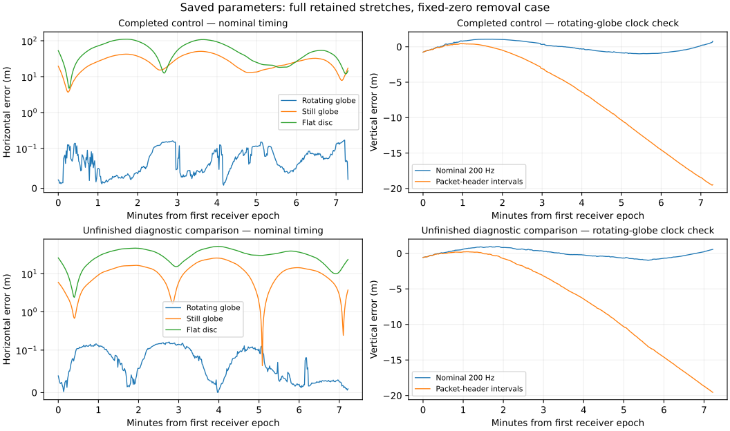
The figure uses the fixed-zero removal case. Its horizontal scale is linear below 0.1 m and logarithmic above it, so centimetre and tens-of-metres errors remain visible together. These are the same observations used to fit the parameters, not held-out predictions.
What individual residuals reveal
- Rotating-globe nominal residuals are small, but remain temporally correlated after the original covariance whitening. Across both stretches and cases, centered lag-one correlations are about 0.42–0.49 north, 0.49–0.59 east and 0.74–0.76 vertically. Receiver intervals are approximately one second; exact lag durations and longer lags are retained in the diagnostic record. A small RMS does not establish independent, correctly modeled errors.
- The largest absolute primary-whitened rotating-globe component under nominal timing is about 0.47; still-globe and flat errors are much larger and have strong temporal structure. No normalized rotating-globe component exceeds three in these checks. This describes the chosen covariance and fitted observations, not a calibrated outlier or adequacy test.
- In the diagnostic stretch, north/east rotating-globe physical errors have rank associations of roughly +0.80/−0.86 with a speed proxy derived from receiver coordinates. Their horizontal RMS is still only about 0.085 m. Such associations can reflect modeling, coordinate rounding or shared measurement errors; they do not identify a physical cause. Altitude, latitude and elapsed time also co-vary along these short routes.
Integration-clock sensitivity
| Stretch / processing case | Nominal vertical RMS (m) | Header vertical RMS (m) | Nominal horizontal RMS (m) | Header horizontal RMS (m) |
|---|---|---|---|---|
| Control / retained | 0.697 | 9.360 | 0.081 | 0.111 |
| Control / removal profiled | 0.697 | 9.360 | 0.081 | 0.111 |
| Diagnostic / retained | 0.559 | 9.233 | 0.085 | 0.106 |
| Diagnostic / removal profiled | 0.562 | 9.261 | 0.085 | 0.106 |
Replacing nominal 200 Hz intervals with packet-header intervals at the same saved parameters raises rotating-globe vertical error to about 9.2–9.4 m. The horizontal model-error separation remains large in these fixed-parameter checks. This does not establish which clock convention is physically correct or what the best refitted header-clock solution would be. A matched, reoptimized clock comparison is the next numerical question; all three candidates must receive the same assumptions and budget.
What is saved and what remains
Axis diagnostics give distributions, signed means, RMS and lag-one correlations for every fit/clock. The compressed per-prediction CSV files alongside this guide preserve every receiver epoch, observed coordinates, coordinate errors, physical errors and primary/conservative whitened innovations. The report record retains 95th/99th percentiles, maxima, longer lags and descriptive rank associations.
The motion proxies are derivatives of receiver coordinates under an explicitly named reference globe metric. They are not the recorded VTG speed samples used for eligibility, nor an independent validation of that metric. Longitude wrapping is preserved in residual calculations. Cholesky innovations use the stacked latitude/longitude/height order; they are not physical north/east/up error magnitudes. No temperature channel is invented.
No absolute-fit acceptance threshold, held-out test or independent uncertainty calibration has been established. No original fit, source, selection or scientific decision is changed. The diagnostic stretch’s small unfinished rotating-globe residual remains useful for solver diagnosis, but it is not a finished model comparison.
Next: specify a small timing/calibration comparison, qualify the revised solver on independent controls, and assess genuine prediction checks. Exact device documentation remains parallel work. See the analysis roadmap.
Reproduction and recovery
The numerical run is complete and frozen. Do not launch it again. Packaging does not make predictions:
env PYTHONPATH=analysis OPENBLAS_NUM_THREADS=2 OMP_NUM_THREADS=2 MKL_NUM_THREADS=2 ~/venv/bin/python analysis/tests/ilvis0_residual_diagnostic.py --package-only
env PYTHONPATH=analysis ~/venv/bin/python docs/ilvis0-residual-diagnostic-20261010/build_report.py
The worker has an exclusive lock, immutable identities, pre-evaluation charges, hashed caches and atomic outputs. Interrupted charged predictions have no automatic retry. The publication receipt verifies numerical outputs; a separate report receipt records this renderer, its input receipt and the generated prose/figure. Neither renderer invokes native prediction.